Blondel's Two Reaction Theory (Theory of Salient Pole Machine)

Blondel's Two Reaction Theory (Theory of Salient Pole Machine) : 
It is known that in case of nonsalient pole type alternators the air gap is uniform. Due to uniform air gap, the field flux as well as armature flux very sinusoidally in the air gap. In nonsalient rotor alternators, air gap length is constant and reactance is also constant. Due to this the m.m.f.s of armature and field act upon the same magnetic circuit all the time hence can be added vectorially. But in salient pole type alternators the length of the air gap varies and the reluctance also varies. Hence the armature flux and field flux cannot vary sinusoidally in the air gap. The reluctances of the magnetic circuits on which m.m.fs act are different in case of salient pole alternators.

       Hence the armature and field m.m.f.s cannot be treated in a simple way as they can be in a nonsalient pole alternators.

       The theory which gives the method of analysis of the distributing effects caused by salient pole construction is called two reaction theory. Professor Andre Blondel has put forward the two reaction theory.

Note : According to this theory the armature m.m.f. can be divided into two components as,

1. Components acting along the pole axis called direct axis
2. Component acting at right angles to the pole axis called quadrature axis.

       The component acting along direct axis can be magnetising or demagnetising. The component acting along quadrature axis is cross magnetising. These components produces the effects of different kinds.

       The Fig. 1 shows the stator m.m.f. wave and the flux distribution in the air gap along direct axis and quadrature axis of the pole.

Fig. 1 Flux distribution in air gap for salient pole machine

       The reluctance offered to the m.m.f. wave is lowest when it is aligned with the field pole axis. This axis is called direct axis of pole i.e. d-axis. The reluctance offered is highest when the m.m.f. wave is oriented at 90 to the field pole axis which is called quadrature axis i.e. q-axis. The air gap is least in the centre of the poles and progressively increases on moving away from the centre. Due to such shape of the pole-shoes, the field winding wound on salient poles produces the m.m.f. wave which is nearly sinusoidal and it always acts along the pole axis which is direct axis.

       Let F_f  be the m.m.f. wave produced by field winding, then it always acts along the direct axis. This m.m.f. is responsible to produce an excitation e.m.f. E_f  which lags F_f  by an angle 90^o .

       When armature carries current, it produces its own m.m.f. wave F_AR. This can be resolved in two components, one acting along d-axis (cross-magnetising). Similarly armature current  I_a  also can be divided into two components, one along direct axis and along quadrature axis. These components are denoted as,

:                   F_d  = Component along direct axis
F_AR :   } 
                    F_q  = Component along quadrature axis

                    I_d  = Component along direct axis
I_a  :    } 
                    I_q  = Component along quadrature axis

       The positions of F_AR, F_d  and F_q  in space are shown in the Fig. 2. The instant chosen to show these positions is such that the current in phase R is maximum positive and is lagging E_f  by angle Ψ.

Fig. 2 M.M.F. wave positions in salient pole machine

       The phasor diagram corresponding to the positions considered is shown in the Fig. 3. The I_a  lags E_f  by angle Ψ.

        It can be observed that F_d  is produced by I_d  which is at 90^o to E_f  while F_q  is produced by I_q  which is in phase with E_f .

       The flux components of Φ_AR which are Φ_d  and Φ_q along the direct and quadrature axis respectively are also shown in the Fig.3. It can be denoted that the reactance offered to flux along direct axis is less than the reactance offered to flux along quadrature axis. Due to this, the flux Φ_AR is no longer along F_AR or I_a. Depending upon the reluctances offered along the direct and quadrature axis, the flux Φ_AR lags behind I_a.

Fig 3  Basic phasor diagram for salient pole machine

We know that, the armature reaction flux Φ_AR has two components, Φ_d along direct axis and Φ_q along quadrature axis. These fluxes are proportional to the respective m.m.f. magnitudes and the permeance of the flux path oriented along the respective axes.

.^..                          Φ_d  = P_d F_d

            where        P_d = permeance along the direct axis

       Permeance is the reciprocal of reluctance and indicates ease with which flux can travel along the path.

       But                 F_d = m.m.f. = K_ar I_d in phase with  I_d 

       The m.m.f. is always proportional to current. While K_ar is the armature reaction coefficient.

.^..                          Φ_d  = P_d K_ar I_d 

       Similarly          Φ_q = P_q K_ar I_q

       As the reluctance along direct axis is less than that along quadrature axis, the permeance  P_d along direct axis is more than that along quadrature axis, (P_d < P_q ).

        Let E_d and E_q be the induced e.m.f.s due to the fluxes Φ_d  and Φ_q respectively. Now E_d lags Φ_d  by 90^o while E_q  lags Φ_q by 90^o .

       where K_e  = e.m.f. constant of armature winding

       The resultant e.m.f. is the phasor sum of E_f, E_d  and E_q.

       Substituting expressions for Φ_d  and Φ_q 

       Now       X_ard  = Equivalent reactance corresponding to the d-axis component of armature reaction

                               = K_e  P_d  K_ar 

       and         X_arq    = Equivalent reactance corresponding to the q-axis component of armature reaction

                                =  K_e  P_q  K_ar 

       For a realistic alternator we know that the voltage equation is,

        where       V_t = terminal voltage

                         X_L  = leakage reactance

       Substituting in expression for Ē_R ,

        where  X_d    = d-axis synchronous reactance = X_L  + X_ard                                   .............(2)

        and      X_q    = q-axis synchronous reactance =  X_L  +  X_arq                                     .........(3)

It can be seen from the above equation that the terminal voltage V_t is nothing but the voltage left after deducing ohmic drop I_a R_a, the reactive drop I_d X_d in quadrature with I_d and the reactive drop I_q X_q  in quadrature with I_d, from the total e.m.f. E_f.

The phasor diagram corresponding to the equation (1) can be shown as in the Fig. 1. The current I_a lags terminal voltage V_t by Φ. Then add I_a R_a in phase with I_a to V_t. The drop I_d X_d leads I_d by 90^o as in case purely reactive circuit current lags voltage by 90^o i.e. voltage leads current by 90^o . Similarly the drop I_q X_q  leads X_q  by 90^o . The total e.m.f. is E_f.

In the phasor diagram shown in the Fig. 4, the angles Ψ and δ are not known, through V_t,  I_a and Φ values are known. Hence the location of E_f is also unknown. The components of I_a, I_d  and I_q  can not be determined which are required to sketch the phasor diagram.

Fig. 4

       Let us find out some geometrical relationships between the various quantities which are involved in the phasor diagram. For this, let us draw the phasor diagram including all the components in detail.

We know from the phasor diagram shown in the Fig. 4 that,

       I_d  =    I_a  sin Ψ                                          ............. (4)

       I_q = I_a cos Ψ                                              ..............(5)

       cosΨ = I_q/I_a                                              ...............(6)

       The drop I_a R_a has two components which are,

        I_d R_d = drop due to R_a in phase with I_d

        I_q R_a = drop due to R_a in phase with I_q

       The I_d X_d and I_q R_q can be drawn leading I_d  and I_q by 90^o respectively. The detail phasor diagram is shown in the Fig. 5.

Fig. 5  Phasor diagram for lagging p.f.

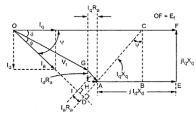
       In the phasor diagram,

      OF =  E_f

      OG =  V_t

      GH =    I_d R_a and H_A = I_q R_a

      GA = I_a R_a

      AE =  I_d X_d and EF = I_q X_a

       Now DAC is drawn perpendicular to the current phasor I_a and CB is drawn perpendicular to AE.

       The triangle ABC is right angle triangle,

       But from equations (6), cosΨ = I_q/I_a

        Thus point C can be located. Hence the direction of E_f is also known.

       Now triangle ODC is also right angle triangle,

       Now OD = OI + ID = V_t cos Φ  + I_a R_a

       and CD = AC + AD = I_a X_q + V_t sinΦ 

       As I_a X_q is known, the angle Ψ can be calculated from equation (10). As Φ is known we can write,

       δ = Ψ - Φ for lagging p.f.

       Hence magnitude of E_f  can be obtained by using equation (11).

Note : In the above relations, Φ is taken positive for lagging p.f. For leading p.f., Φ must be taken negative.